CME

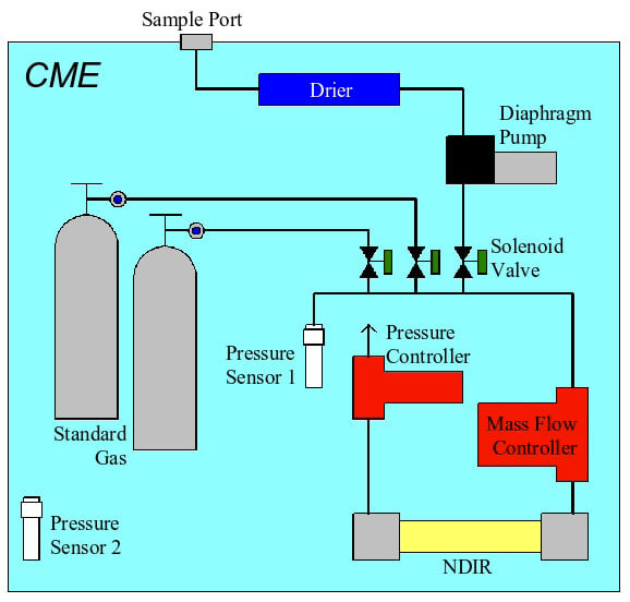
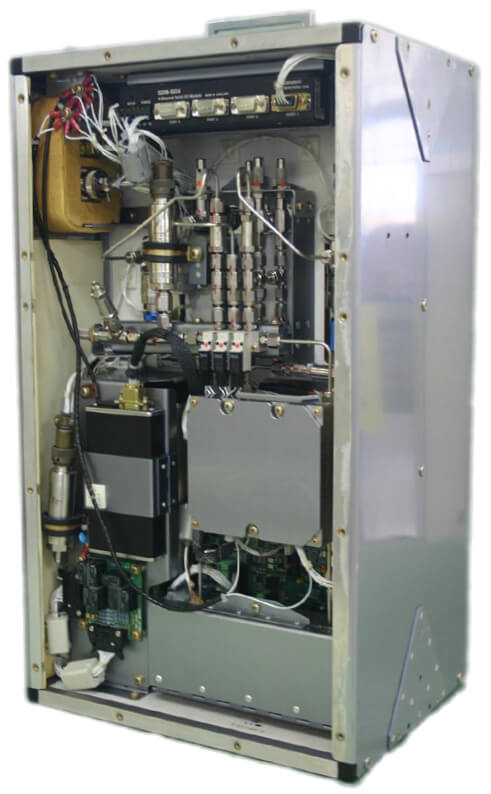
Figure 1 shows a schematic diagram of the CME package (264 mm length x 330 mm width x 570 mm height), which weighs about 25 kg. The main components are a drier, a pump, solenoid valves, a flow controller, a pressure controller, NDIR analyzer (LICOR, LI-840), two standard gas cylinders, and a programmable controller/datalogger device (Figure 2). Air samples are drawn by a diaphragm pump from the intake port mounted on the air conditioning duct and then introduced into the analyzer. In the upstream of the pump, a drier tube packed with CO₂-saturated magnesium perchlorate is used to remove water vapor. The flow rate of the sampled air into the NDIR cell is kept constant at 150 standard cc per minute (sccm) by a mass flow controller. In addition, the absolute pressure of the sampled air in the NDIR cell is maintained at 0.110 MPa by an auto pressure controller to avoid signal drift in the NDIR associated with changes in cabin pressure.

Navigation data received by the controller/datalogger device include date, time, pressure altitude, radio altitude, latitude, longitude, ground speed, static air temperature, and wind direction and velocity. In order to avoid sampling of heaviliy polluted air (high CO₂ and H₂O) in the lower layers of the atmosphere, air sampling does not start until the radio altitude registers 2000 feet during the ascent, and stops at 2000 feet during the descent. All of the data from the aircraft data system, the NDIR signal, flow rate, cell pressure and supplied air pressure measured by pressure sensor 1 are recorded every 10 seconds during the ascent and descent and every 1 minute during the level flight. The time interval of 10 seconds corresponds to about 100m in altitude, while that of 1 minute corresponds to 10-20 km in the horizontal. The measurement precision is estimated to be 0.1 ppm (one standard deviation) when using 10-second averaged data. Thus, CME enables us to resolve the fine structures of the atmospheric CO₂ distribution from all of the flights (Machida et al. 2008).

Latitudinal distributions of CO₂ measured by CME in the upper troposphere between Sydney and Narita are compared in Figure 3 with those obtained by ASE during the December 8, 2005 flight. Both data are in a good agreement, i.e. within ±0.2ppm. Data from other flights carrying ASE and CME show likewise good agreements. Analytical precision and accuracy are relatively better for ASE since flask samples are analyzed by a LI-6252 (LICOR) in our laboratory under controlled conditions. Therefore, the data agreement indicates a high reliability in CO₂ measurements by a small NDIR inside the CME.

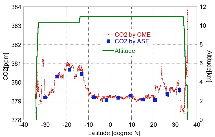
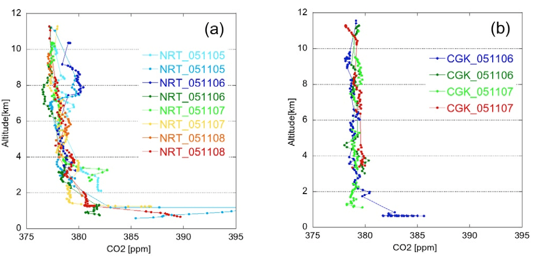
Figure 4 shows vertical CO₂ distributions obtained over Narita, Japan (NRT) and Jakarta, Indonesia (CGK) on 5–8 November 2005. High CO₂ values near the surface reflect CO₂ contaminated by human activities around the airport. Vertical profiles in the free troposphere are tightly bound over both airports, indicating high reproducibility of CME observation. The vertical gradient with higher CO₂ mixing ratios at the lower altitudes over NRT (Figure 4a) is caused by CO₂ release from land vegetation and fossil fuel use in this area. On the other hand, relatively constant CO₂ with height over CGK is reflective of the wide tropical region where net surface CO₂ emissions are weak and vertical air mixing is efficient; these observation results are similar to results from a previous aircraft observation campaign (Machida et al. 2003).

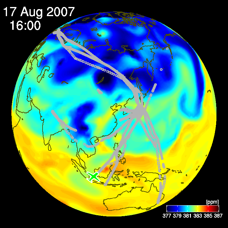
Distribution of CO₂ in the atmosphere varies with meteorology. Figure 5 (Click to view) illustrates an example of how CO₂ distribution at the cruising altitude (about 10 km) changes during a month together with when and where our aircraft measured CO₂. The CO₂ distirbutions were computed by an atmospheric transport model (Niwa et al. 2012)

After 10 years of CME measurements, we obtained > 7 million CO₂ data points from > 12 thousand flights. In particular, we have the highest data density over the Asia-Pacific region. The numerous data enabled us seasonal climatology of CO₂ distribution well visualized horizontally and vertically over Asia (Figure 6).

References

- Machida, T., K. Kita, Y. Kondo, D. Blake, S. Kawakami, G. Inoue, and T. Ogawa, (2003), J. Geophys. Res., 108(D3), doi:10.1029/2001JD000910.
- Machida, T., H. Matsueda, Y. Sawa, et al., (2008), Worldwide measurements of atmospheric CO2 and other trace gas species using commercial airlines. J. Atmos. Oceanic. Technol., 25 (10), 1744-1754, DOI: 10.1175/2008JTECHA1082.1.
- Niwa, Y., T. Machida, Y. Sawa, H. Matsueda, T. J. Schuck, C. A. M. Brenninkmeijer, R. Imasu, and M. Satoh (2012), Imposing strong constraints on tropical terrestrial CO2 fluxes using passenger aircraft based measurements, J. Geophys. Res., 117(D11303), doi:10.1029/2012JD017474.
- Umezawa, T., H. Matsueda, Y. Sawa, Y. Niwa, T. Machida, and L. Zhou (2018), Seasonal evaluation of tropospheric CO2 over the Asia-Pacific region observed by the CONTRAIL commercial airliner measurements, Atmos. Chem. Phys., 18, 14851–14866, doi:10.5194/acp-18-14851-2018.