Collected Data of High Temporal-Spatial Resolution Marine Biogeochemical Monitoring from Ferries in the East Asian Marginal Seas (April 1994–December 1995)
 |
This CD-ROM contains the data of a marine environmental monitoring program using 2 ferries, which followed up the previous Japan-Korea Ferry monitoring between Pusan and Kobe1)-3) carried out in 1991-1993 (hereinafter referred to as Line (a)).
The new program is using 2 ferry cruise tracks : Line (b)Osaka - Seto Inland Sea - Beppu and Line (c) Osaka - Kuroshio Current - Okinawa.
The policy of the newly selected geographical coverage is to take over the time series for the Seto Inland Sea part of Line(a) by implementing (b) and to cover the zonation structure between the inner bay - shelf slope - oligotrophic Kuroshio Current by implementing Line (c).
It also includes computer-generated images that will help the users visualize the temporal-spatial variations of the parameters.
1. Introduction
Increases in the extent of human activities have strongly impacted the cycling of elements such as C, N, and P. The changes in these cycles would occur first in the marginal seas and the establishment of monitoring systems to assess such changes is urgently needed, particularly in the waters neighboring the Asian countries.
To comprehend the mechanisms and processes of environmental changes, monitoring programs with the following characteristics should be implemented: (1) long duration, (2) sampling frequency sufficient to resolve phenomena over various spatial and temporal scales, (3) linkage with satellite missions, particularly those with ocean color sensors7), (4) robustness of the methods, (5) linkage with modeling efforts, (6) minimization of costs, (7) quick processing and distribution of the data products in both numerical and graphic form, and (8) holistic approach for the comprehensive understanding of ecosystem health.
Biogeochemical monitoring using the sea water intake of ferries was evaluated with respect to these needs and found to be feasible. We developed a prototype system in 1990 and deployed it on a ship track on Line (a) (Fig.1). The procedures necessary for such monitoring have been described in other reports1),2). The initial numerical data and image files were published in a CD-ROM3) and distributed to pertinent organizations including the Japan Oceanographic Data Center (JODC). One can browse the contents of the CD-ROM at the CGER world wide web site, URL: http://www.cger.nies.go.jp/publications/report/d007/d007-e.html
The ferry service sailing Line (a) ceased operation in 1993. Therefore, new ferry tracks were selected based on the criteria discussed below.
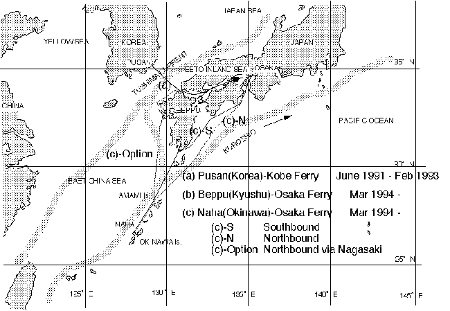
Fig. 1 Ferry cruise tracks used for monitoring. The previous Japan-Korea Ferry Program used Line (a). The present program is being carried out on Lines (b) and (c).
2. Geographical Coverage of the Monitoring
The program since 1994 has been based on the following 2 ferry tracks.
Line (b) traverses the Seto Inland Sea, a characteristic semi-enclosed sea heavily affected by anthropogenic impacts. Line (c) traverses the zonation structure from a semi-enclosed sea, across the shelf slope, and into the Kuroshio Current. Both ships belong to Kansai Kisen Co., Ltd. Thus the combination of results from these 2 lines facilitates assessment of both anthropogenic trends and background characteristics. The latter role was played in part by the Tsushima Strait portion of the Line (a) cruise track. The Tsushima Current stems from the subtropical gyre in the area around Okinawa and Kyushu and flows in this strait, entraining the water of the East China Sea.
On Line (c), the southbound and northbound tracks differ from each other because the ship takes advantage of the northeast-component of the Kuroshio when sailing north, but avoids it by taking a route nearer to the coast on the southward leg. Furthermore, several northbound cruises sail a course in the East China Sea via Nagasaki for special cruises (Fig. 1).
3. Measurement Methods
The equipment and methods used on Line (b) (Fig. 2) are basically identical to those used on Line (a).
Water temperature(T), salinity (S), pH, and dissolved oxygen were obtained by integrated water quality
sensors (Hydrolab H20). The in vivo fluorescence was measured by a Turner Design Fluorometer.
Automated filtration sampling for dissolved nutrients, chlorophyll-a, and phaeopigments was done at 24
points every other week only on Line (b). The weekly maintenance (retrieval of the data and samples and
calibration and readjustment of the sensors) was done while the ships were at Osaka Port. An inventory
of the data from these 2 series of cruises are listed in the APPENDIX.TXT file on the CD-ROM. All other
differences between the methods used on Lines (b) and (c) are listed in Table 1.
Table.1 Difference between the methods for Line (b) and (c).
| Track Line | (b)Osaka - Seto Inland Sea | (c)Osaka-Okinawa |
| Ship | Sunflower-2 | Ferry Kuroshio |
| Cruise frequency | 1 one-say cruise/nightly | 1 round-trip / weekly |
| Sea water source | engine-cooling system | another valve |
| Cruise duration | 12 hours | 44 hours |
| Sensor measurements every 10 seconds | T, S, pH, (Dissolved-O2) in vivo Fluorescence | same |
| Unattended filtration sampling at every other week(24 samples) | NO3, NO2, NH4, PO4, Si(OH)4, chlorophyll-a, phaeopigments | none |
Furthermore, attended investigations were occasionally carried out on both ferry lines to perform research-oriented experiments or optional measurements simultaneous with regular monitoring. Although the results of such supplemental measurements are omitted here and left for individual research publications5),6), the dates and lists of measured variables from supplemental measurements are listed in the APPENDIX.TXT file on the CD-ROM.
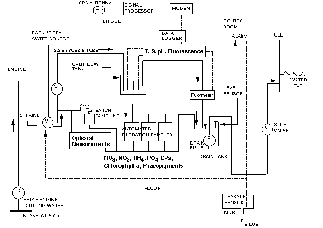
Fig. 2 Monitoring system deployed on (b) the Osaka-Beppu line (Sunflower 2).
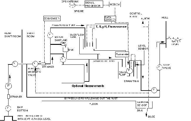 The system on (c), the Osaka-Okinawa line (Ferry Kuroshio), is similar to this one.
However, the sea water on Ferry Kuroshio is not from the engine cooling system but rather from a recently installed valve, unlike that on Line (b), and no automatic filtration sampling is conducted.
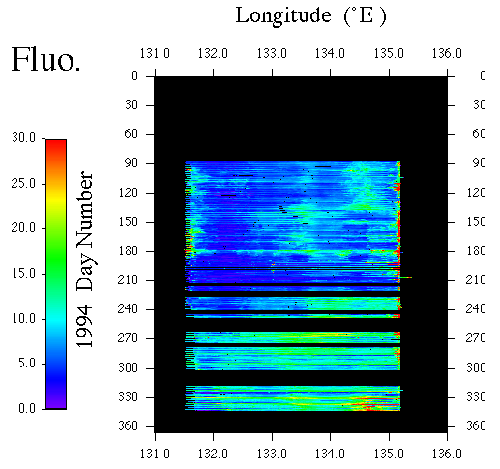
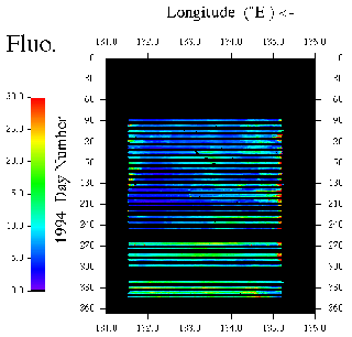
Fig. 3 Examples of computer generated images of the temporal-spatial variation of in vivo fluorescence for 1994 created from Level-2 data from cruises sailing in both directions ( image files FLU94 on this CD ). The vertical axis shows the day number from January 1 to December 31 downward. The horizontal axis shows the longitude between Beppu (left) and Osaka (right).
 |
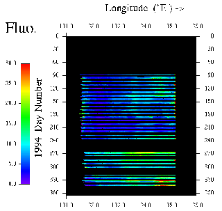 |
| The images (b) and (c) were created from westbound cruise only, and eastbound cruise only, respectively (image files FLU94W and FLU94E, respectively, on this CD ). | |
4. Data Processing
Details of the regular monitoring methods are shown in other reports1),2),4) and some points are briefly
repeated here. The sensor signals more or less drift to some extent over the course of each week of
continuous flow-through measurements due to the gradual fouling of their seaward-facing surfaces.
Therefore, the data were processed as follows. At first, Level-1 data is generated as a text file
converted from the raw binary data. Level-2 data of T, S, in vivo fluorescence, and DO were then
computed by correcting the Level-1 data with the calibration values for before and after each weekly
measuring period, assuming that the fouling is linear with time. This CD-ROM contains Level-2 data, each
numerical file of which corresponds to a one-way cruise.
Two kinds of corrected data of pH were generated. Using only the calibration value for before each week of continuous measurements, the pH1 data series was generated without temperature correction. Using the calibration values for before and after each week, the pH2 data series was generated assuming that water temperature was 25 deg. and that sensor drift was linear with time during the continuous measurements.
While we include oxygen values for reference, their accuracy can not be assured because the one week cruise durations exceeded the expected life of the probe membranes. The fluorescence values are recorded in units of fluoresceine solution (used for calibration) equivalent concentrations . Based on the correlation between them, the chlorophyll-a concentration (in microgram kg-1) was around 1/4 of the fluorescence value. The quality of the Level-2 fluorescence data was sometimes degraded by non-linear drift of the sensor with time. Especially, the data in the oligotrophic part of Line(c) could not be validated. However, they were not omitted because they would contribute in a sense of relative values to the analysis of phytoplankton patchness or the frontal structure.
Images such as those in (e.g., Fig. 3 for in vivo fluorescence in 1994) were generated to comprehensively reveal the temporal-spatial variation of variables. To produce such images, a text matrix was generated so that each row expresses the spatial distribution obtained from each cruise and each column expresses the temporal variation. The dimensions corresponding to each pixel of the images for Line (b) are 0.5deg. latitude by 1 day Line (b). In the case of Line (c), each pixel corresponds to 0.5deg. longitude by 1 day. The text matrix was color-processed with Spyglass R. Discretely sampled data, such as that for nutrients, are also processed as temporal-spatial maps.
To some extent, in vivo fluorescence from eastbound cruises (Osaka Bay in the evening and Beppu in the morning) differed systematically from those on the westbound cruises (reverse chronology). In vivo fluorescence was higher in the morning than in the evening (see Fig. 3(b) and (c)). There are 2 possible causes for this pattern, both related to the circadian rhythm of phytoplankton. One is the diurnal cycle of the biomass-specific fluorescence intensity and the other is vertical migration of motile phytoplankton. Thus the temporal-spatial resolution achieved in the present monitoring has the potential to reveal in situ physiology or dynamics of phytoplankton.
In spite of certain insufficiencies of the Level-2 data, we conclude that they are quite informative and valuable. The absolute accuracy of the Level-2 data will be improved by retrospective correction against data of point measurements from the usual research vessels. We will generate Level-3 data via such processes as the next step.
5. Data files and Directories on these CD-ROM
This CD-ROM can be mounted on DOS, UNIX, and Macintosh platforms provided with ISO9660 compatible CD-Mounters.
A synopsis of the CD-ROM is shown in README.TXT, which is almost identical to this booklet and included in the
SYNOPSIS-directory. APPENDIX.TXT contains Appendix 1.(directory structure), Appendix 2.(an inventory of the
monitoring cruises) and Appendix 3 ( a list of attended investigation cruises ). They are seen in more
orderly form if imported to a word processor with tabsets at every 1 cm and courier fonts of 10points than
are read as a raw text.
The FIGURE-directory contains figures such as Figs. 1 and 2. The NUMDATA directory contains the subdirectories BTFL94 and BTFL95, which contain the DOS-text files from automated filtration sampling. Each subdirectory, L2Y94M04, ...., L2Y95M12, contains the Level-2 data for each month. Macintosh computer users can transform DOS-text to Mac-text by changing [CR LF] to [CR] with the TM Apple File Exchange utility.
One record (line) of each bottle and filter data file consists of date+time (date by I6 + L.S.T. by I4), latitude (degree by I2 + minutes by F4.1), longitude (degree by I3 + minutes by F4.1), filtered water volume (ml), dissolved nutrients (micro M) (Dissolved-Si, PO4-P, NH4-N, NO2-N, NO2+NO3-N, and NO3-N), chlorophyll-a (microgram/l), phaeopigments (microgram/l), where I and F refer to integers and floating point values, respectively.
The Level-2 Data files for each cruise consist of approximately 4300 and 13000 data records for Lines (b) and (c), respectively. One record line corresponds to 1 measurement every 10 seconds and contains the date, local time, cumulative date from 1900, longitude, latitude, pH1, salinity (per mille), water temperature (deg.), fluorescence (equivalent concentration of fluoresceine, microgram/l), dissolved oxygen (mg/l), pH2, error flags for the H-20 sensors, Turner Design fluorometer, and GPS, respectively. The flag value 0 means no trouble. The IMAGE-directory contains the image files such as those presented in Fig. 3. Here, the file name FLU95E (FLU95W) denotes the images of the fluorescence data processed from only the eastbound (westbound) cruises on Line (b). In the same manner, the images processed from data of the southbound (northbound) cruises of Line (c) have file names such as FLU94S (FLU94N). These image files were savedin GIF (*.GIF) format. The text matrix generated for processing tempo al-spatial maps is contained in a subdirectory named WSHEET under NUMDATA.
6. Acknowledgments
This project owes much of its success to the cooperation of the Kansai Kisen Co., Ltd.
The project has been implemented by the participants in the Monitoring Execution Group and
Organizations listed below, based on discussions of the Committee for East Asian Ferry Monitoring,
which has been organized by NIES-CGER, and the subcommittee's advisory members.
Committee for East Asian Ferry Monitoring:
R.Tsuda (8) ( Chair ), A.Harashima(1)(12), K.Kohata(12), Y.Nojiri(1)(12), K.Ohta(11), K.Takano#, H.Takeoka(3)
Secretariat Office:
N.Furuta(1), Y.Fujinuma(1), S.Fukuzawa(1), T.Ukigai(1), Y.Yoichi(1), T.Fukushima(1)
Monitoring Execution Team:
A.Harashima(1)(12)( Chief ), T.Hagiwara(2), H.Kimoto(7), T.Kimoto(7) (13), S.Sakamoto(4), Y.Tanaka(8), H.Tatsuta(4), T.Toshiyasu(4), T.Wakabayashi(4)
Advisory members:
H.-D.Ahn(9), K.Imao(10), K.Furusawa(10), Y.Furukawa(5), M.Kunugi(12), Y.Nakamura(12), J.-R.Oh(9), S.Tanaka(6)
CD-ROM Making Team:
A.Harashima(1)(12), Y.Satoh(12), S.Nakai(1), T.Miyazaki(1)
Participating Organizations:
NIES-CGER(1), Global Environmental Forum(2), Ehime University(3), JWA(Japan Weather Association)(4), Kansai Kisen Co., Ltd.(5), Keio University(6),
Kimoto Electric Co., Ltd.(7), Kinki University(8), KORDI(Korea Ocean Research and Development Institute)(9), Marine Biological Research Institute of Japan,
Co., Ltd.(10), Nagoya University(11), NIES(12), RIOC(Research Institute of Oceano-Chemistry)(13) , Professor Emeritus of University of Tsukuba#.
References
1)Harashima, A. (1993 ): Annual Report on Global Environmental Monitoring 1993, CGER-M003-'93, 33-45.
2)Harashima, A. (1994): Monitoring Report on Global Environment 1994, CGER-M004-'94, 13-50.
3)Harashima, A. (ed.) (1995): Collected data of high temporal-spatial resolution marine biogeochemical monitoring by Japan-Korea ferry boat-June 1991-February 1993-, CGER-D007(CD-ROM)-'95.
4)Harashima, A. (1995): Monitoring Report on Global Environment 1995, CGER-M005-'95, 21-38.
5)Harashima, A., R. Tsuda, Y. Tanaka, T. Kimoto, K. Furusawa and H. Tatsuta,(1997):Mati Kahru ( ed. ) Monitoring Algal Blooms: New Techniques for Detecting Large-Scale Environmental Change, ( to be published, R. G. Landes Bioscience Publishers and Academic Press ).
6)Kimoto, K. and A. Harashima (1993): Proc. 4th Internat.CO2 Conf. WMO, Global Atmosphere Watch 89, 88-91.
7)Harashima, A. and Y. Kikuchi, (1990): EOS, 10, 314-315.